Stream input data

import warnings

import cartopy
import cartopy.crs as ccrs
import matplotlib as mpl
import matplotlib.pyplot as plt

import tams

warnings.filterwarnings("ignore", category=cartopy.io.DownloadWarning)

GPM precipitation and brightness temperature

With the help of earthaccess, we can stream these data without downloading the files to disk.

• tams.data.get_imerg()

• tams.data.get_mergir()

%%time

pr = tams.data.get_imerg("2024-06-01 02:30")["pr"]
pr

CPU times: user 620 ms, sys: 199 ms, total: 819 ms
Wall time: 9.59 s

<xarray.DataArray 'pr' (lat: 1800, lon: 3600)> Size: 26MB
[6480000 values with dtype=float32]
Coordinates:
    time     datetime64[ns] 8B 2024-06-01T02:30:00
  * lon      (lon) float32 14kB -179.9 -179.9 -179.8 ... 179.8 179.8 179.9
  * lat      (lat) float32 7kB -89.95 -89.85 -89.75 -89.65 ... 89.75 89.85 89.95
Attributes:
    units:        mm/hr
    long_name:    precipitation rate
    description:  Complete merged microwave-infrared (gauge-adjusted) precipi...

xarray.DataArray

'pr'

• lat: 1800
• lon: 3600

• ...

  [6480000 values with dtype=float32]

• Coordinates: (3)
  • time
    ()
    datetime64[ns]
    2024-06-01T02:30:00

    array('2024-06-01T02:30:00.000000000', dtype='datetime64[ns]')

  • lon
    (lon)
    float32
    -179.9 -179.9 ... 179.8 179.9

    units :

    degrees_east

    long_name :

    longitude

    description :

    Longitude at the center of 0.10 degree grid intervals of longitude from -180 to 180.

    array([-179.95   , -179.85   , -179.75   , ...,  179.75   ,  179.84999,
            179.95   ], shape=(3600,), dtype=float32)

  • lat
    (lat)
    float32
    -89.95 -89.85 ... 89.85 89.95

    units :

    degrees_north

    long_name :

    latitude

    description :

    Latitude at the center of 0.10 degree grid intervals of latitude from -90 to 90.

    array([-89.95, -89.85, -89.75, ...,  89.75,  89.85,  89.95],
          shape=(1800,), dtype=float32)

• Indexes: (2)
  • lon
    PandasIndex

    PandasIndex(Index([ -179.9499969482422, -179.85000610351562,             -179.75,
           -179.64999389648438,  -179.5500030517578,  -179.4499969482422,
           -179.34999084472656,             -179.25, -179.14999389648438,
            -179.0500030517578,
           ...
             179.0500030517578,  179.14999389648438,              179.25,
            179.34999084472656,   179.4499969482422,   179.5500030517578,
            179.64999389648438,              179.75,  179.84999084472656,
             179.9499969482422],
          dtype='float32', name='lon', length=3600))

  • lat
    PandasIndex

    PandasIndex(Index([-89.94999694824219,  -89.8499984741211,             -89.75,
            -89.6500015258789, -89.54999542236328, -89.44999694824219,
            -89.3499984741211,             -89.25,  -89.1500015258789,
           -89.04999542236328,
           ...
            89.04999542236328,   89.1500015258789,              89.25,
             89.3499984741211,  89.44999694824219,  89.54999542236328,
             89.6500015258789,              89.75,   89.8499984741211,
            89.94999694824219],
          dtype='float32', name='lat', length=1800))

• Attributes: (3)

  units :

  mm/hr

  long_name :

  precipitation rate

  description :

  Complete merged microwave-infrared (gauge-adjusted) precipitation estimate; formerly precipitationCal

%%time

tb = tams.data.get_mergir(pr.time.item())["tb"]
tb

CPU times: user 76.5 ms, sys: 28.8 ms, total: 105 ms
Wall time: 17.1 s

<xarray.DataArray 'tb' (lat: 3298, lon: 9896)> Size: 131MB
[32637008 values with dtype=float32]
Coordinates:
  * lon      (lon) float32 40kB -180.0 -179.9 -179.9 ... 179.9 179.9 180.0
  * lat      (lat) float32 13kB -59.98 -59.95 -59.91 ... 59.91 59.95 59.98
    time     datetime64[ns] 8B 2024-06-01T02:30:00
Attributes:
    units:          K
    standard_name:  brightness_temperature
    long_name:      brightness temperature

xarray.DataArray

'tb'

• lat: 3298
• lon: 9896

• ...

  [32637008 values with dtype=float32]

• Coordinates: (3)
  • lon
    (lon)
    float32
    -180.0 -179.9 ... 179.9 180.0

    units :

    degrees_east

    standard_name :

    longitude

    long_name :

    longitude

    array([-179.98181, -179.94543, -179.90906, ...,  179.90906,  179.94543,
            179.98181], shape=(9896,), dtype=float32)

  • lat
    (lat)
    float32
    -59.98 -59.95 ... 59.95 59.98

    units :

    degrees_north

    standard_name :

    latitude

    long_name :

    latitude

    array([-59.981808, -59.945423, -59.909035, ...,  59.90904 ,  59.945423,
            59.981808], shape=(3298,), dtype=float32)

  • time
    ()
    datetime64[ns]
    2024-06-01T02:30:00

    standard_name :

    time

    array('2024-06-01T02:30:00.000000000', dtype='datetime64[ns]')

• Indexes: (2)
  • lon
    PandasIndex

    PandasIndex(Index([ -179.9818115234375,  -179.9454345703125,  -179.9090576171875,
            -179.8726806640625,  -179.8363037109375,  -179.7999267578125,
           -179.76353454589844, -179.72715759277344, -179.69078063964844,
           -179.65440368652344,
           ...
             179.6544189453125,   179.6907958984375,   179.7271728515625,
             179.7635498046875,   179.7999267578125,   179.8363037109375,
             179.8726806640625,   179.9090576171875,   179.9454345703125,
             179.9818115234375],
          dtype='float32', name='lon', length=9896))

  • lat
    PandasIndex

    PandasIndex(Index([-59.981807708740234,   -59.9454231262207, -59.909034729003906,
           -59.872650146484375, -59.836265563964844,  -59.79988098144531,
           -59.763492584228516, -59.727108001708984,  -59.69072341918945,
           -59.654335021972656,
           ...
             59.65433883666992,   59.69072341918945,  59.727108001708984,
            59.763492584228516,   59.79987716674805,   59.83626937866211,
             59.87265396118164,   59.90903854370117,    59.9454231262207,
            59.981807708740234],
          dtype='float32', name='lat', length=3298))

• Attributes: (3)

  units :

  K

  standard_name :

  brightness_temperature

  long_name :

  brightness temperature

%%time

fig = plt.figure(figsize=(12, 5), layout="constrained")
ax = fig.add_subplot(projection=ccrs.PlateCarree())

ax.coastlines(color="magenta")

cmap = plt.get_cmap("gist_gray_r")
cmap.set_bad("red")
tb.plot(x="lon", cmap=cmap, robust=True, ax=ax)
pr.plot(x="lon", norm=mpl.colors.LogNorm(0.01, pr.quantile(0.99)), alpha=0.85, ax=ax);

CPU times: user 7.64 s, sys: 3.49 s, total: 11.1 s
Wall time: 16 s

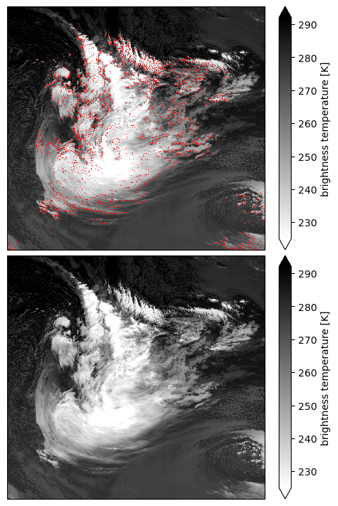
The red dots in the brightness temperature field above represent missing data. For most CE identification methods, this will influence results. Since they are mostly scattered points, not large regions, a reasonable way to fill in the missing data is a nearest-neighbor interpolation.

%%time

kws = dict(method="nearest", fill_value="extrapolate", assume_sorted=True)
tb_ = tb.interpolate_na("lat", **kws).interpolate_na("lon", **kws)

print(f"{tb.isnull().sum().item() / tb.size:.3%} -> {tb_.isnull().sum().item() / tb_.size:.3%} null")

2.231% -> 0.000% null
CPU times: user 1.1 s, sys: 97.4 ms, total: 1.2 s
Wall time: 10.4 s

We zoom in to the system off the coast of Chile to demonstrate the impact.

box = dict(lon=slice(-115, -80), lat=slice(-53, -20))

fig, [ax1, ax2] = plt.subplots(
    2, 1,
    figsize=(5, 7),
    sharex=True, sharey=True,
    subplot_kw=dict(projection=ccrs.Mercator()),
    layout="constrained",
)

tb.sel(box).plot(cmap=cmap, robust=True, ax=ax1)
ax1.set_title("")

tb_.sel(box).plot(cmap=cmap, robust=True, ax=ax2)
ax2.set_title("");