Identify

Here, we demonstrate the impacts of some of the tams.identify() options.

import matplotlib.pyplot as plt
import xarray as xr

import tams

xr.set_options(display_expand_data=False)

Show code cell output

Hide code cell output

<xarray.core.options.set_options at 0x7ec58261d550>

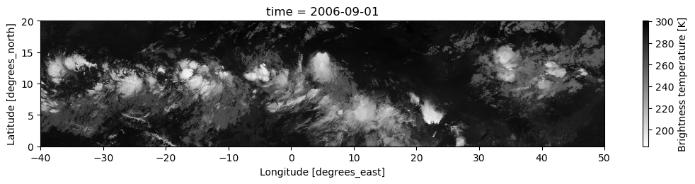
tb = tams.load_example_tb().isel(time=0)

tb.plot(x="lon", y="lat", size=2.3, aspect=6, cmap="gist_gray_r")

ax = plt.gca()
ax.set(xlim=(-40, 50), ylim=(0, 20))
ax.set_aspect("equal", "box")

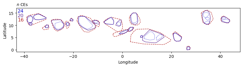
Contour thresholds

fig, ax = plt.subplots(figsize=(10, 3))

for i, (thresh, color, ls) in enumerate(
    [
        (250, "firebrick", "--"),
        (235, "rebeccapurple", "-"),  # default
        (225, "mediumblue", ":"),
    ]
):
    ce = tams.identify(tb, ctt_threshold=thresh)[0][0]
    ce.plot(ax=ax, ec=color, fc="none", ls=ls)
    ax.text(0.005, 0.98 - (2 - i) * 0.1, len(ce), color=color, size=12, ha="left", va="top", transform=ax.transAxes)

ax.set_title("$n$ CEs", loc="left", size=10)
ax.set(xlabel="Longitude", ylabel="Latitude");

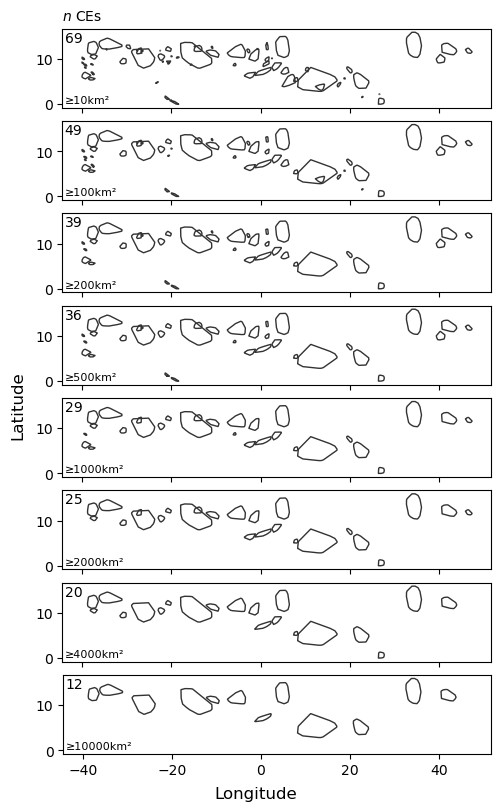
Size filtering threshold

%%time

cases = [10, 100, 200, 500, 1000, 2000, 4000, 10_000]

fig, axs = plt.subplots(len(cases), 1, sharex=True, sharey=True, figsize=(5, 8), constrained_layout=True)

for ax, thresh in zip(axs.flat, cases):
    ce = tams.identify(tb, size_threshold=thresh)[0][0]
    ce.plot(ax=ax, ec="0.2", fc="none")
    ax.text(0.005, 0.97, f"{len(ce)}", size=10, ha="left", va="top", transform=ax.transAxes)
    ax.text(0.005, 0.03, f"≥{thresh}km²", size=8, ha="left", va="bottom", transform=ax.transAxes)

axs[0].set_title("$n$ CEs", loc="left", size=10)
fig.supxlabel("Longitude")
fig.supylabel("Latitude");

CPU times: user 3.27 s, sys: 35.9 ms, total: 3.31 s
Wall time: 3.31 s

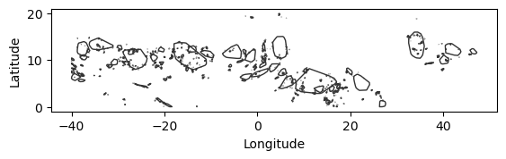
Disabling size filtering completely is possible but generally not useful except for debugging, or if you want to do your own size filtering. (Tiny CEs, that would otherwise be filtered out, are often too small to be linked with area overlap methods.) Also note that CE areas, needed by tams.classify(), are not computed by tams.identify() when size filtering is disabled.

(
    tams.identify(tb, size_filter=False)[0][0]
    .plot(ec="0.2", fc="none")
    .set(xlabel="Longitude", ylabel="Latitude")
);