MPAS unstructured grid data#
In this example, we demonstrate CE identification with unstructured-grid data from MPAS-A and compare to the results using the regridded dataset.
import warnings

import cartopy.io
import cartopy.crs as ccrs
import cartopy.feature as cfeature
import geopandas as gpd
import matplotlib as mpl
import matplotlib.pyplot as plt
import numpy as np
import pandas as pd
import xarray as xr
from matplotlib.tri import Triangulation

import tams

warnings.filterwarnings("ignore", category=cartopy.io.DownloadWarning)

%matplotlib inline

xr.set_options(display_expand_data=False)
Load data#
ds = tams.data.open_example("mpas-native")
ds
<xarray.Dataset> Size: 138MB
Dimensions:  (time: 127, cell: 133447)
Coordinates:
  * time     (time) datetime64[ns] 1kB 2006-09-08T12:00:00 ... 2006-09-13T18:...
    lat      (cell) float64 1MB ...
    lon      (cell) float64 1MB ...
Dimensions without coordinates: cell
Data variables:
    tb       (time, cell) float32 68MB ...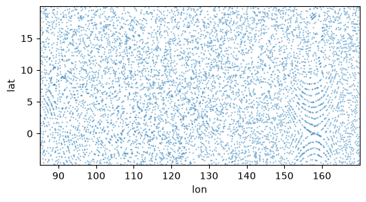
pr (time, cell) float32 68MB ...fig, ax = plt.subplots(figsize=(6, 3))
sel = ds.isel(cell=slice(None, None, 20))
ax.scatter(sel.lon, sel.lat, marker=".", s=10, alpha=0.5, edgecolors="none")
ax.set(xlabel="lon", ylabel="lat")
ax.autoscale(tight=True)
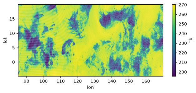
%%time

fig, ax = plt.subplots(figsize=(7.5, 3))

im = ax.scatter(ds.lon, ds.lat, c=ds.tb.isel(time=10), marker=".", s=3, edgecolors="none")
fig.colorbar(im, ax=ax, label="Tb")
ax.autoscale(tight=True)
ax.set(xlabel="lon", ylabel="lat");
CPU times: user 331 ms, sys: 153 ms, total: 483 ms
Wall time: 483 ms
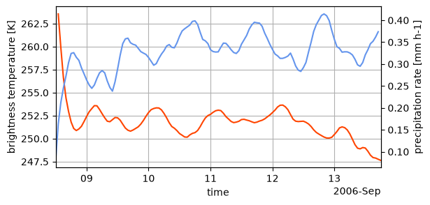
ts = ds.mean("cell", keep_attrs=True)

fig, ax = plt.subplots(figsize=(6, 3))
ax2 = ax.twinx()

ts.tb.plot(ax=ax, c="orangered")
ts.pr.plot(ax=ax2, c="cornflowerblue")
ax.autoscale(axis="x", tight=True)
ax.grid(True)
Identify CEs#
%%time

itime = 10

stime = pd.Timestamp(ds.time.values[itime]).strftime(r"%Y-%m-%d_%H")
print(stime)

x = ds.lon
y = ds.lat
tri = Triangulation(x, y)
2006-09-08_22
CPU times: user 882 ms, sys: 37.6 ms, total: 920 ms
Wall time: 921 ms
%%time

# Passing the triangulation in is not required but makes it faster
shapes = (
    tams.contour(ds.tb.isel(time=itime), value=235, triangulation=tri)
    .pipe(tams.core._contours_to_polygons)
);
CPU times: user 442 ms, sys: 1.64 ms, total: 443 ms
Wall time: 446 ms
%%time

# `tams.identify` does the above but also for the core threshold and does size filtering by default
(ce_ug,) = tams.identify(ds.tb.isel(time=itime))
CPU times: user 1.69 s, sys: 142 ms, total: 1.83 s
Wall time: 1.82 s
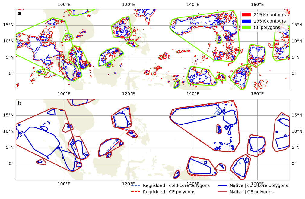
%%time

tran = ccrs.PlateCarree()
proj = ccrs.PlateCarree()  # near equator

fig, (ax1, ax2) = plt.subplots(2, 1, figsize=(10, 6), subplot_kw=dict(projection=proj), constrained_layout=True)

ax = ax1

ax.add_feature(cfeature.LAND)

tcs = ax.tricontour(tri, ds.tb.isel(time=itime), levels=[235], colors="red", linewidths=1, transform=tran)
tcs_core = ax.tricontour(tri, ds.tb.isel(time=itime), levels=[219], colors="blue", linewidths=1, transform=tran)

shapes.plot(fc="none", ec="green", lw=1.5, ls=":", ax=ax, transform=tran)  # not size-filtered
ce_ug.plot(fc="none", ec="lawngreen", lw=2, ax=ax, zorder=3, transform=tran)

ax.gridlines(draw_labels=True)

legend_handles = [
    mpl.patches.Patch(color="red", label="219 K contours"),
    mpl.patches.Patch(color="blue", label="235 K contours"),
    mpl.patches.Patch(color="lawngreen", label="CE polygons"),
]
ax.legend(handles=legend_handles, loc="upper right")

ax = ax2

ds_rg = tams.data.open_example("mpas-regridded").sel(lat=slice(None, 20))  # same lat upper bound as in the ug data

ax.add_feature(cfeature.LAND)

(ce_rg,) = tams.identify(ds_rg.tb.isel(time=itime))

a = ce_rg.core.plot(fc="none", ec="royalblue", lw=1.5, ls="--", transform=tran, ax=ax)
ce_ug.core.plot(fc="none", ec="mediumblue", lw=2, transform=tran, ax=ax)

ce_rg.plot(fc="none", ec="red", lw=1.5, ls="--", transform=tran, ax=ax)
ce_ug.plot(fc="none", ec="firebrick", lw=2, zorder=3, transform=tran, ax=ax)

legend_handles = [
    mpl.lines.Line2D([], [], color="royalblue", ls="--", lw=1.5, label="Regridded | cold-core polygons"),
    mpl.lines.Line2D([], [], color="red", ls="--", lw=1.5, label="Regridded | CE polygons"),
    mpl.lines.Line2D([], [], color="mediumblue", ls="-", lw=2, label="Native | cold-core polygons"),
    mpl.lines.Line2D([], [], color="firebrick", ls="-", lw=2, label="Native | CE polygons"),
]

gl = ax.gridlines(draw_labels=True)
gl.top_labels = False
# ax.autoscale(tight=True)
ax.set_xlim(ax1.get_xlim()); ax.set_ylim(ax1.get_ylim())
fig.legend(handles=legend_handles, ncol=2, loc="lower right", bbox_to_anchor=[0, -0.09, 0.961, 1], frameon=False)

for a, ax in zip("abc", [ax1, ax2]):
    ax.text(0.007, 0.98, a, weight="bold", size=14, va="top", ha="left", transform=ax.transAxes)

fig.savefig(f"mpas-ug-contours-and-vs-rg-ces_{stime}.pdf", bbox_inches="tight", pad_inches=0.05, transparent=False)
CPU times: user 2.28 s, sys: 122 ms, total: 2.4 s
Wall time: 5.85 s
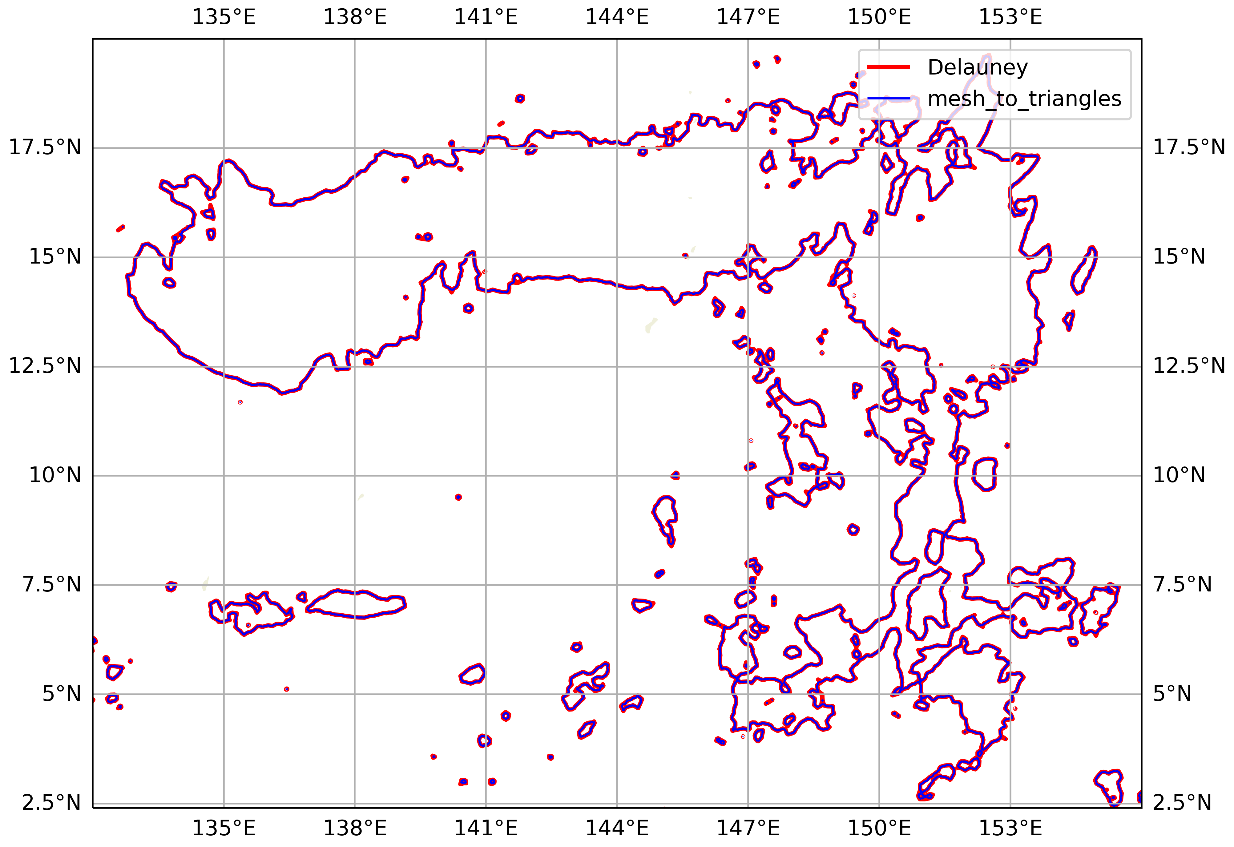
Triangulations#
The above contouring is based on the Delauney triangulation. This connects the cell centers with straight lines to form triangles. But this triangulation doesn’t correspond to the MPAS mesh, per se.
MPAS-Tools, though, provides a method for dividing the mesh grid cells into triangles and interpolating data defined at cell centers (like OLR) to the triangle nodes. The triangle nodes include the cell centers (one per triangle) and the grid cell vertices (two per triangle). A hexagonal grid cell, e.g., is divided into 6 triangles, which all share the cell center as a node.
We compared the contourings from these two methods. For our intents and purposes (identifying CEs with area ≥ 4000 km²), the differences appear to be negligible. The mesh horizontal resolution is 15 km, which seems to be sufficiently high that the Delauney triangulation is a good approximation.
# Code
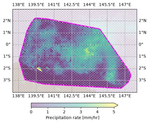
Precip inside CE#
This figure is intended to demonstrate what tams.data_in_contours() does.
one_ce = ce_ug.cx[138:145, -4:3]
assert len(one_ce) == 1, "just one CE"

fig, ax = plt.subplots(figsize=(5, 4), subplot_kw=dict(projection=proj), constrained_layout=True)

ax.gridlines(draw_labels=True)
ax.set_extent([137.5, 148, -4, 3], crs=tran)
ax.add_feature(cfeature.LAND)

# tcs = ax.tricontourf(tri, ds.tb.isel(time=itime), levels=20, cmap="viridis_r", transform=tran)

pr = ds.pr.isel(time=itime)
s = ax.scatter(pr.lon, pr.lat, c=pr,
    ec="none", s=7,
    cmap="viridis", vmin=0, vmax=5, alpha=0.35,
    transform=tran,
)

within = (
    gpd.GeoDataFrame({"pr": pr}, geometry=gpd.points_from_xy(pr.lon, pr.lat, crs=4326))
    .sjoin(one_ce[["geometry"]], predicate="within", how="left")
    .dropna(subset="index_right")
)
within.plot(ax=ax, column="pr", cmap="viridis", vmin=0, vmax=5, markersize=12, edgecolor="none")

one_ce.plot(ax=ax, fc="none", ec="magenta", lw=2)

# one_ce.set_geometry("core").plot(ax=ax, fc="none", ec="cyan", lw=1.5)

fig.colorbar(s, orientation="horizontal", extend="max", shrink=0.7, label="Precipitation rate [mm/hr]")

fig.savefig(f"mpas-ug-points-within-example_{stime}.png", dpi=200, bbox_inches="tight", pad_inches=0.05, transparent=False)
Versions#
%load_ext watermark
%watermark -v -w -p cartopy,dask,gdown,geopandas,joblib,matplotlib,netCDF4,numpy,pandas,regionmask,scipy,seaborn,shapely,skimage,xarray
Python implementation: CPython
Python version       : 3.14.6
IPython version      : 9.15.0

cartopy   : 0.25.0
dask      : 2026.7.0
gdown     : 6.1.0
geopandas : 1.1.4
joblib    : 1.5.3
matplotlib: 3.11.0
netCDF4   : 1.7.4
numpy     : 2.4.6
pandas    : 2.3.3
regionmask: 0.13.0
scipy     : 1.18.0
seaborn   : 0.13.2
shapely   : 2.1.2
skimage   : 0.26.0
xarray    : 2026.7.0

Watermark: 2.6.0