Stream input data

import warnings

import cartopy.io
import cartopy.crs as ccrs
import matplotlib.pyplot as plt
import xarray as xr
from matplotlib.colors import LogNorm

import tams

warnings.filterwarnings("ignore", category=cartopy.io.DownloadWarning)

xr.set_options(display_expand_data=False)

Show code cell output

Hide code cell output

<xarray.core.options.set_options at 0x7101c6a9eba0>

GPM precipitation and brightness temperature

With the help of earthaccess, we can stream these data without downloading the files to disk.

• tams.data.get_imerg()

• tams.data.get_mergir()

%%time

if HAVE_AUTH:
    pr = tams.data.get_imerg("2024-06-01 02:30")["pr"]
else:
    pr = tams.data.load_example("docs-get-example-imerg")["pr"]

pr

/home/docs/checkouts/readthedocs.org/user_builds/tams/conda/latest/lib/python3.14/site-packages/earthaccess/results.py:348: FutureWarning: As of version 1.0, `DataGranule.size` will be accessed as an attribute; e.g. use `DataCollection.size` **not** `DataCollection.size()`
  self["size"] = self.size()
/home/docs/checkouts/readthedocs.org/user_builds/tams/conda/latest/lib/python3.14/site-packages/earthaccess/store.py:523: FutureWarning: As of version 1.0, `DataGranule.size` will be accessed as an attribute; e.g. use `DataCollection.size` **not** `DataCollection.size()`
  total_size = round(sum([granule.size() for granule in granules]) / 1024, 2)

CPU times: user 757 ms, sys: 400 ms, total: 1.16 s
Wall time: 7.6 s

<xarray.DataArray 'pr' (lat: 1800, lon: 3600)> Size: 26MB
...
Coordinates:
  * lat      (lat) float32 7kB -89.95 -89.85 -89.75 -89.65 ... 89.75 89.85 89.95
  * lon      (lon) float32 14kB -179.9 -179.9 -179.8 ... 179.8 179.8 179.9
    time     datetime64[ns] 8B 2024-06-01T02:30:00
Attributes:
    units:        mm/hr
    long_name:    precipitation rate
    description:  Complete merged microwave-infrared (gauge-adjusted) precipi...

xarray.DataArray

'pr'

• lat: 1800
• lon: 3600

• ...

  [6480000 values with dtype=float32]

• Coordinates: (3)
  • lat
    (lat)
    float32
    -89.95 -89.85 ... 89.85 89.95

    units :

    degrees_north

    long_name :

    latitude

    description :

    Latitude at the center of 0.10 degree grid intervals of latitude from -90 to 90.

    array([-89.95, -89.85, -89.75, ...,  89.75,  89.85,  89.95],
          shape=(1800,), dtype=float32)

  • lon
    (lon)
    float32
    -179.9 -179.9 ... 179.8 179.9

    units :

    degrees_east

    long_name :

    longitude

    description :

    Longitude at the center of 0.10 degree grid intervals of longitude from -180 to 180.

    array([-179.95   , -179.85   , -179.75   , ...,  179.75   ,  179.84999,
            179.95   ], shape=(3600,), dtype=float32)

  • time
    ()
    datetime64[ns]
    2024-06-01T02:30:00

    array('2024-06-01T02:30:00.000000000', dtype='datetime64[ns]')

• Attributes: (3)

  units :

  mm/hr

  long_name :

  precipitation rate

  description :

  Complete merged microwave-infrared (gauge-adjusted) precipitation estimate; formerly precipitationCal

%%time

if HAVE_AUTH:
    tb = tams.data.get_mergir(pr.time.item())["tb"]
else:
    tb = tams.data.load_example("docs-get-example-mergir")["tb"]

tb

/home/docs/checkouts/readthedocs.org/user_builds/tams/conda/latest/lib/python3.14/site-packages/earthaccess/results.py:348: FutureWarning: As of version 1.0, `DataGranule.size` will be accessed as an attribute; e.g. use `DataCollection.size` **not** `DataCollection.size()`
  self["size"] = self.size()
/home/docs/checkouts/readthedocs.org/user_builds/tams/conda/latest/lib/python3.14/site-packages/earthaccess/store.py:523: FutureWarning: As of version 1.0, `DataGranule.size` will be accessed as an attribute; e.g. use `DataCollection.size` **not** `DataCollection.size()`
  total_size = round(sum([granule.size() for granule in granules]) / 1024, 2)

CPU times: user 144 ms, sys: 35.8 ms, total: 180 ms
Wall time: 6.53 s

<xarray.DataArray 'tb' (lat: 3298, lon: 9896)> Size: 131MB
[32637008 values with dtype=float32]
Coordinates:
  * lat      (lat) float32 13kB -59.98 -59.95 -59.91 ... 59.91 59.95 59.98
  * lon      (lon) float32 40kB -180.0 -179.9 -179.9 ... 179.9 179.9 180.0
    time     datetime64[ns] 8B 2024-06-01T02:30:00
Attributes:
    units:          K
    standard_name:  brightness_temperature
    long_name:      brightness temperature

xarray.DataArray

'tb'

• lat: 3298
• lon: 9896

• ...

  [32637008 values with dtype=float32]

• Coordinates: (3)
  • lat
    (lat)
    float32
    -59.98 -59.95 ... 59.95 59.98

    units :

    degrees_north

    standard_name :

    latitude

    long_name :

    latitude

    array([-59.981808, -59.945423, -59.909035, ...,  59.90904 ,  59.945423,
            59.981808], shape=(3298,), dtype=float32)

  • lon
    (lon)
    float32
    -180.0 -179.9 ... 179.9 180.0

    units :

    degrees_east

    standard_name :

    longitude

    long_name :

    longitude

    array([-179.98181, -179.94543, -179.90906, ...,  179.90906,  179.94543,
            179.98181], shape=(9896,), dtype=float32)

  • time
    ()
    datetime64[ns]
    2024-06-01T02:30:00

    standard_name :

    time

    array('2024-06-01T02:30:00.000000000', dtype='datetime64[ns]')

• Attributes: (3)

  units :

  K

  standard_name :

  brightness_temperature

  long_name :

  brightness temperature

%%time

fig = plt.figure(figsize=(12, 5), layout="constrained")
ax = fig.add_subplot(projection=ccrs.PlateCarree())

ax.coastlines(color="magenta")

cmap = plt.get_cmap("gist_gray_r")
cmap.set_bad("red")
tb.plot(x="lon", cmap=cmap, robust=True, ax=ax)
pr.plot(x="lon", norm=LogNorm(0.01, pr.quantile(0.99)), alpha=0.85, ax=ax);

CPU times: user 7.91 s, sys: 3.02 s, total: 10.9 s
Wall time: 13.4 s

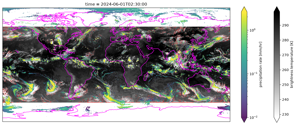
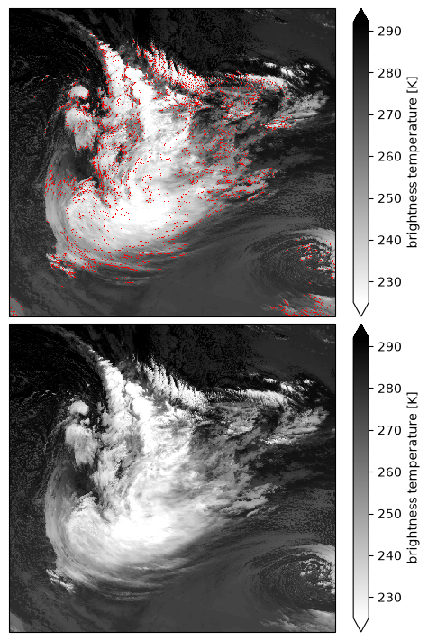
The red dots in the brightness temperature field above represent missing data. For most CE identification methods, this will influence results. Since they are mostly scattered points, not large regions, a reasonable way to fill in the missing data is a nearest-neighbor interpolation.

%%time

kws = dict(method="nearest", fill_value="extrapolate", assume_sorted=True)
tb_ = tb.interpolate_na("lat", **kws).interpolate_na("lon", **kws)

print(f"{tb.isnull().sum().item() / tb.size:.3%} -> {tb_.isnull().sum().item() / tb_.size:.3%} null")

2.231% -> 0.000% null
CPU times: user 1.6 s, sys: 61.1 ms, total: 1.66 s
Wall time: 1.92 s

We zoom in to the system off the coast of Chile to demonstrate the impact.

box = dict(lon=slice(-115, -80), lat=slice(-53, -20))

fig, [ax1, ax2] = plt.subplots(
    2, 1,
    figsize=(5, 7),
    sharex=True, sharey=True,
    subplot_kw=dict(projection=ccrs.Mercator()),
    layout="constrained",
)

tb.sel(box).plot(cmap=cmap, robust=True, ax=ax1)
ax1.set_title("")

tb_.sel(box).plot(cmap=cmap, robust=True, ax=ax2)
ax2.set_title("");