Idealized data

Here, we demonstrate the capabilities of tams.idealized for creating synthetic datasets for testing and experimentation.

import warnings

import cartopy.io
import geopandas as gpd
import matplotlib.pyplot as plt

import tams
from tams.idealized import Blob, Field, Sim

warnings.filterwarnings("ignore", category=cartopy.io.DownloadWarning)

Blob

A Blob is an ellipse with parameters tendencies (set to zero by default) and a parabolic well.

The default Blob is a circle.

Blob().polygon

Blob().ring

Blob().to_geopandas().plot();

_, ax = plt.subplots(layout="constrained", figsize=(4, 4))

ax.add_patch(Blob().to_patch(fc="forestgreen"))
ax.set_aspect("equal")
ax.autoscale()

The default Blob has zero tendency in its parameters, meaning that when evolve() is called, it won’t move or grow.

Blob().get_tendency()

{'center': array([0., 0.]),
 'width': 0.0,
 'height': 0.0,
 'angle': 0.0,
 'depth': 0.0}

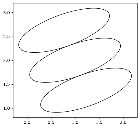
Split

Blob(center=(1, 2)).split()

[Blob(center=[1.   1.75], width=0.5, height=0.5, angle=0),
 Blob(center=[1.   2.25], width=0.5, height=0.5, angle=0)]

Field(Blob(center=(1, 2), width=6, height=2, angle=20).split(3)).to_geopandas().plot(fc="none");

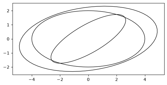
Merge

b1 = Blob(width=6, height=2, angle=30)
b2 = Blob(width=8, height=4)
b3 = b1.merge(b2)

Field([b1, b2, b3]).to_geopandas().plot(fc="none");

Field

A Field is a collection of Blobs on a grid that, together, combine to make a field that we can run tams.identify() on.

Field()

Field(blobs=[])

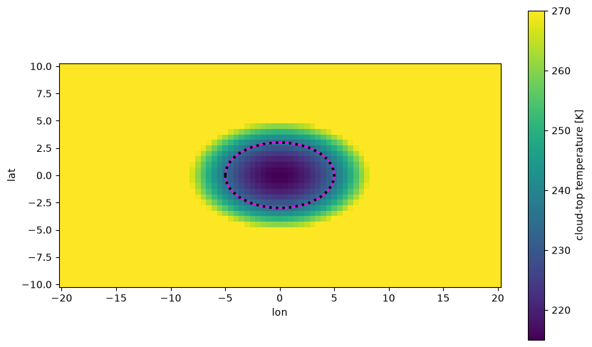
Single well

%%time

b = Blob(center=(0, 0), width=10, height=6)

ctt = Field(b).to_xarray()

(ce,) = tams.identify(ctt)

fig, ax = plt.subplots(figsize=(10, 6))

ctt.plot(ax=ax)
gpd.GeoSeries(b.ring).plot(ec="magenta", ax=ax)

ce.plot(ax=ax, lw=2.5, ls=":", ec="black", fc="none", zorder=10)

ax.set_aspect("equal")

CPU times: user 471 ms, sys: 184 ms, total: 655 ms
Wall time: 983 ms

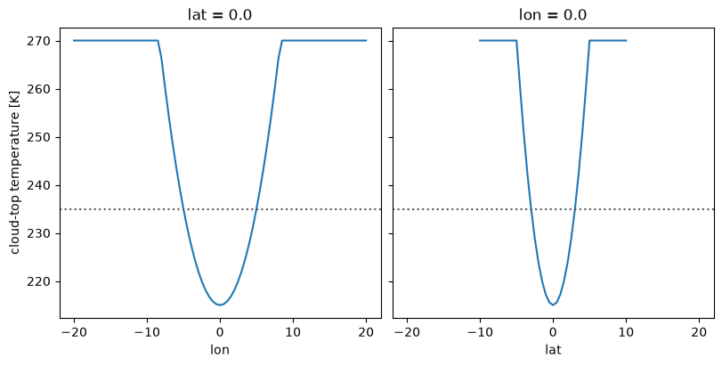
fig, [ax1, ax2] = plt.subplots(1, 2, figsize=(8, 4), sharex=True, sharey=True, layout="constrained")

ctt.sel(lat=0, method="nearest").plot(ax=ax1)
ctt.sel(lon=0, method="nearest").plot(ax=ax2)

ax2.set_ylabel("")
for ax in fig.get_axes():
    ax.axhline(235, c="0.35", ls=":")

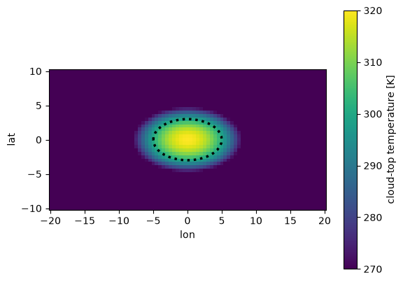
Reverse well

# Flipping depth and making CTT threshold greater than the background,
# we can get a reverse well.
ctt = Field(
    Blob(center=(0, 0), width=10, height=6, depth=-20)
).to_xarray(ctt_threshold=300)

# TAMS will still identify if we adjust the thresholds accordingly
(ce,) = tams.identify(ctt, ctt_threshold=300, ctt_core_threshold=310)

fig, ax = plt.subplots()

ctt.plot(ax=ax)
ce.plot(ax=ax, lw=2.5, ls=":", ec="black", fc="none");

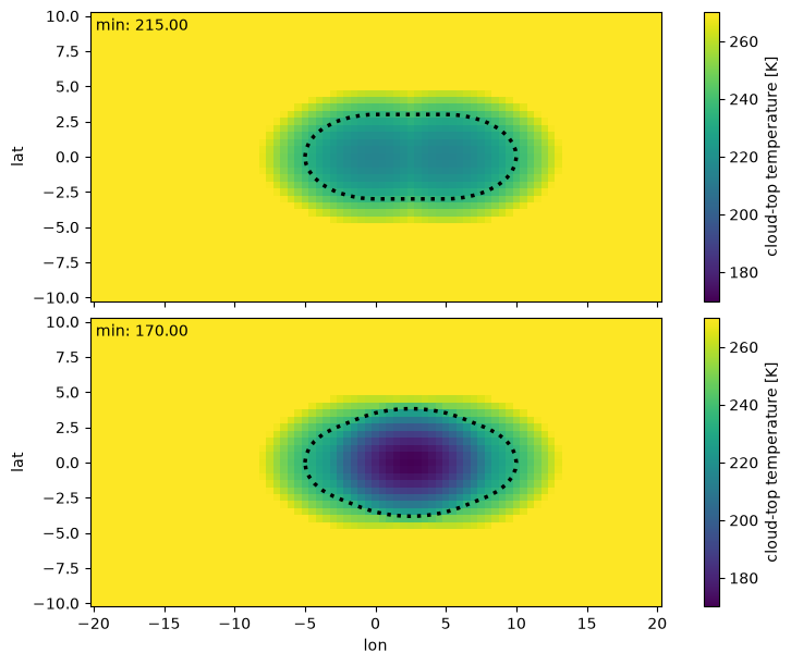
Additive

fld = Field(
    [
        Blob(center=(0, 0), width=10, height=6),
        Blob(center=(5, 0), width=10, height=6),
    ]
)

fig, [ax1, ax2] = plt.subplots(2, 1, figsize=(8, 6), sharex=True, sharey=True, layout="constrained")

kws = dict(vmin=170, vmax=270)
for ax, ctt in zip([ax1, ax2], [fld.to_xarray(), fld.to_xarray(additive=True)]):
    ctt.plot(ax=ax, **kws)
    ax.text(0.01, 0.98, f"min: {ctt.min().item():.2f}", ha="left", va="top", transform=ax.transAxes)
    (ce,) = tams.identify(ctt)
    ce.plot(ax=ax, lw=2.5, ls=":", ec="black", fc="none")

ax1.set_xlabel("")

for ax in [ax1, ax2]:
    ax.set_aspect("equal")

Sim

A Sim is the evolution of a Field in time.

# Nothing (no blobs)
Sim().advance(2).to_xarray().plot(col="time");

%%time

ctt = Sim(
    Field(
        [
            Blob(width=10).set_tendency(center=(2, 0)),
            Blob(center=(-20, -10), width=6).set_tendency(center=(5, 3), width=1),
        ],
        lat=(-15, 15, 61),
    ),
).advance(9).to_xarray()

ces = tams.identify(ctt)

fg = ctt.plot(col="time", cmap="inferno_r", col_wrap=5, aspect=1.35)
for ce, ax in zip(ces, fg.axs.flat):
    if not ce.empty:
        ce.plot(ax=ax, lw=2, ec="w", fc="none")

<timed exec>:11: UserWarning: No CEs identified for time steps: [8, 9]

CPU times: user 2.38 s, sys: 73.8 ms, total: 2.45 s
Wall time: 2.45 s

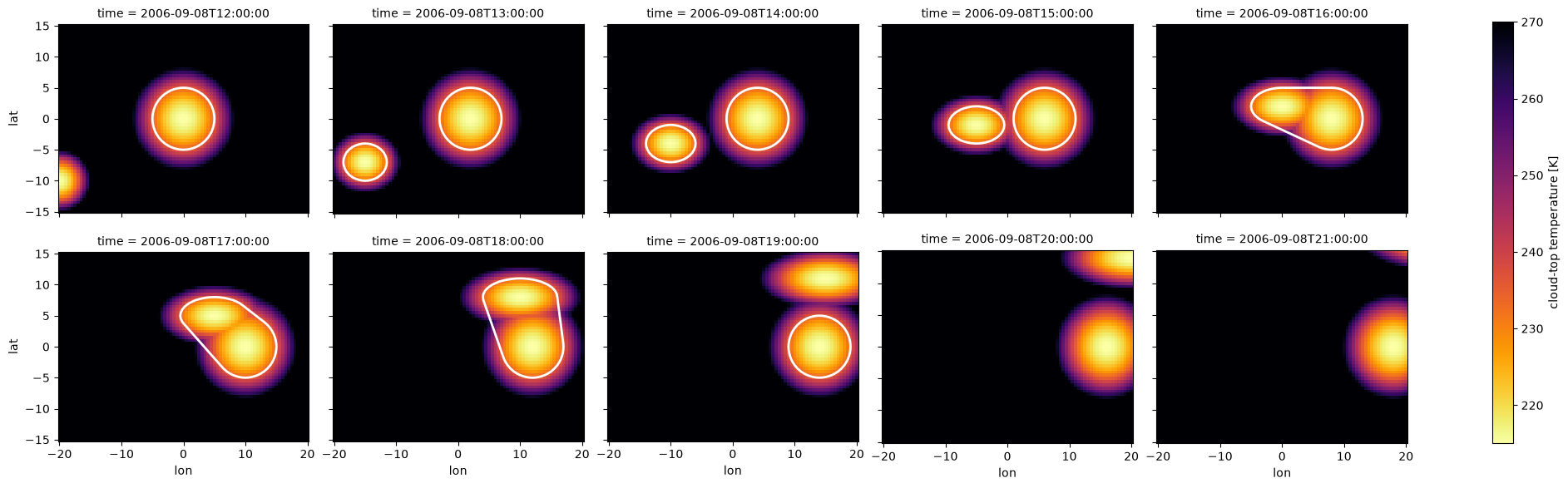
👆 In TAMS v0.2, we lose track of the system(s) the last few time steps because the blobs are partially out of the domain and we drop open contours by default in the identify() stage. In this example, we could fix this by increasing the domain size when creating the Field.

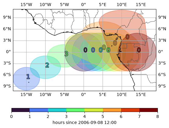
tams.plot_tracked(
    tams.track(ces, ctt.time),
    size=5,
    alpha=0.35,
    add_colorbar=True,
    cmap="turbo",
)