Identify

Here, we demonstrate the impacts of some of the tams.identify() options.

import matplotlib.pyplot as plt
import xarray as xr

import tams

xr.set_options(display_expand_data=False)

Show code cell output

Hide code cell output

<xarray.core.options.set_options at 0x70aad7f6b8c0>

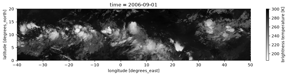
tb = tams.data.open_example("msg-tb")["tb"].isel(time=0).load()

tb.plot(x="lon", y="lat", size=2.3, aspect=6, cmap="gist_gray_r")

ax = plt.gca()
ax.set(xlim=(-40, 50), ylim=(0, 20))
ax.set_aspect("equal", "box")

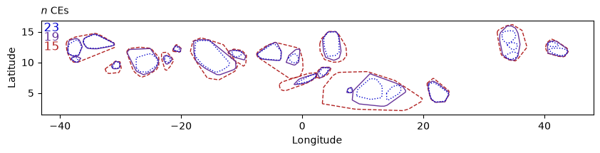
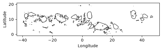
Contour thresholds

fig, ax = plt.subplots(figsize=(10, 3))

for i, (thresh, color, ls) in enumerate(
    [
        (250, "firebrick", "--"),
        (235, "rebeccapurple", "-"),  # default
        (225, "mediumblue", ":"),
    ]
):
    ce = tams.identify(tb, ctt_threshold=thresh)[0]
    ce.plot(ax=ax, ec=color, fc="none", ls=ls)
    ax.text(0.005, 0.98 - (2 - i) * 0.1, len(ce), color=color, size=12, ha="left", va="top", transform=ax.transAxes)

ax.set_title("$n$ CEs", loc="left", size=10)
ax.set(xlabel="Longitude", ylabel="Latitude");

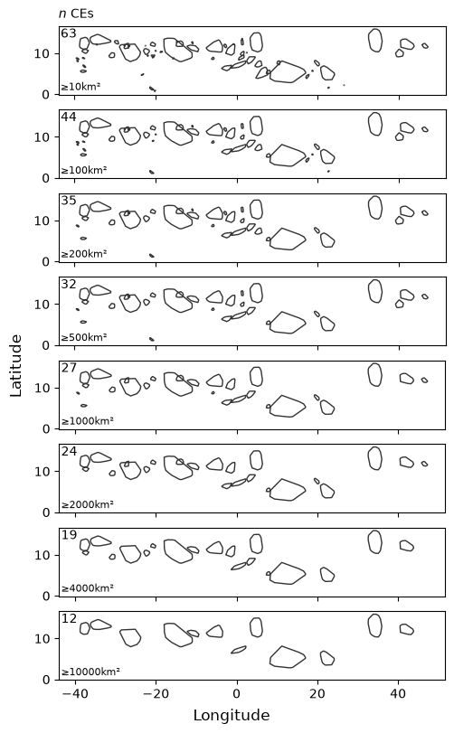
Size filtering threshold

%%time

cases = [10, 100, 200, 500, 1000, 2000, 4000, 10_000]

fig, axs = plt.subplots(len(cases), 1, sharex=True, sharey=True, figsize=(5, 8), constrained_layout=True)

for ax, thresh in zip(axs.flat, cases):
    ce = tams.identify(tb, size_threshold=thresh)[0]
    ce.plot(ax=ax, ec="0.2", fc="none")
    ax.text(0.005, 0.97, f"{len(ce)}", size=10, ha="left", va="top", transform=ax.transAxes)
    ax.text(0.005, 0.03, f"≥{thresh}km²", size=8, ha="left", va="bottom", transform=ax.transAxes)

axs[0].set_title("$n$ CEs", loc="left", size=10)
fig.supxlabel("Longitude")
fig.supylabel("Latitude");

CPU times: user 8 s, sys: 154 ms, total: 8.15 s
Wall time: 8.15 s

Disabling size filtering completely is possible but generally not useful except for debugging, or if you want to do your own size filtering. (Tiny CEs, that would otherwise be filtered out, are often too small to be linked with area overlap methods.) Also note that CE areas, needed by tams.classify(), are not computed by tams.identify() when size filtering is disabled.

(
    tams.identify(tb, size_threshold=0)[0]
    .plot(ec="0.2", fc="none")
    .set(xlabel="Longitude", ylabel="Latitude")
);

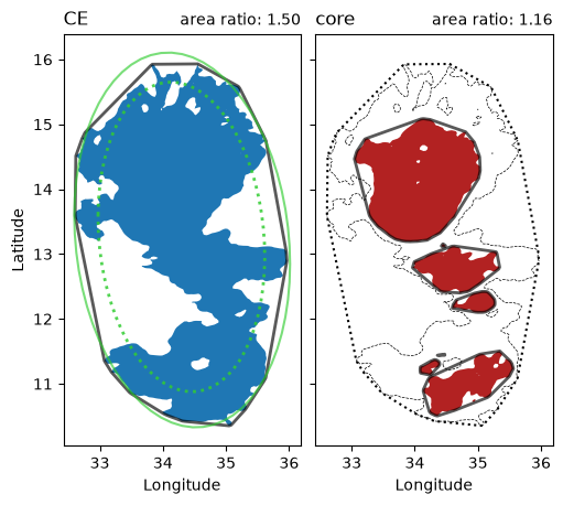
Convex hull

In v0.2 it is possible to disable convex hulling. Using the convex hull gives us a simpler and more efficient shape, but we lose some accuracy in the representation of the field and inflate the area. With convex_hull=False in tams.identify(), we get polygons, based on the closed contours, that account for holes (holes are filled when convex hull is applied).

lat, lon = tb.lat, tb.lon
box = (lat >= 10) & (lat <= 16) & (lon >= 32) & (lon <= 36)

ce = tams.identify(tb.where(box))[0]
ce_no_convex = tams.identify(tb.where(box), convex_hull=False)[0]
assert len(ce) == len(ce_no_convex) == 1

fig, axs = plt.subplots(1, 2, sharex=True, sharey=True, figsize=(5, 5), layout="constrained")

ax = axs.flat[0]
ce_no_convex.plot(fc="C0", ax=ax)
ell_no_convex = tams.fit_ellipse(ce_no_convex.geometry.iat[0])
ell_no_convex.to_blob().to_geopandas().plot(ls=":", ec="limegreen", fc="none", lw=2, alpha=0.85, ax=ax)
ce.plot(fc="none", lw=2, alpha=0.65, ax=ax)
ell = tams.fit_ellipse(ce.geometry.iat[0])
ell.to_blob().to_geopandas().plot(ec="limegreen", fc="none", lw=1.5, alpha=0.65, ax=ax)
ax.set_title("CE", loc="left")
f = (ce.area_km2 / ce_no_convex.area_km2).item()
ax.set_title(f"area ratio: {f:.2f}", loc="right", size=10)
ax.set(xlabel="Longitude", ylabel="Latitude")
print(f"𝑒 (convex hull,    solid):  {ell.eccentricity:.3f}")
print(f"𝑒 (no convex hull, dashed): {ell_no_convex.eccentricity:.3f}")

ax = axs.flat[1]
ce_no_convex.core.plot(fc="firebrick", ax=ax)
ce.core.plot(fc="none", lw=2, alpha=0.65, ax=ax)
ce.plot(fc="none", lw=1.5, ls=":", ax=ax)
ce_no_convex.plot(fc="none", lw=0.5, ls="--", ax=ax)
ax.set_title("core", loc="left")
f = (ce.area_core_km2.sum() / ce_no_convex.area_core_km2.sum()).item()
ax.set_title(f"area ratio: {f:.2f}", loc="right", size=10)
ax.set(xlabel="Longitude", ylabel=None);

𝑒 (convex hull,    solid):  0.813
𝑒 (no convex hull, dashed): 0.838